01. Architecture Overview
GCMS simulates an entire satellite constellation. Each satellite runs as its own process on a server, just as real satellite software runs independently on separate spacecraft. Each process models the satellite's orbit, power system, attitude (orientation), thermal state, communications, and propulsion.
A central operations server discovers these satellite processes automatically, collects their data once per second, and presents everything in the web interface you see. Think of it like a real mission control room that polls telemetry from a fleet of spacecraft.
Deep dive: process architecture
The operations server discovers satellite processes by scanning a range of
TCP ports every 2 seconds, probing each for a /api/v1/health
endpoint. When a satellite responds, it is added to the fleet roster.
The simulation is deterministic given initial orbital elements and runs in accelerated time. All physics models use SI units internally with double-precision (float64) arithmetic. The web client fetches a JSON snapshot of the full constellation at 1 Hz and interpolates between snapshots for smooth display updates.
Practical example: Suppose you launch 30 Galileo satellites.
Each one starts as an independent process listening on its own port
(e.g., GSAT0101 on port 8081, GSAT0102 on port 8082, …). The operations
server scans ports 8081–8144 and finds 30 responding processes. It then
polls GET /api/v1/health on each one every second, receiving
a JSON blob with orbit position, battery charge, thermal temps, etc. If you
kill GSAT0102's process, it disappears from the fleet table within 2 seconds.
Restart it, and it reappears — the operations server doesn't care about
the order or timing of satellite startup.
Each satellite carries metadata from a fleet configuration file: orbital slot (e.g. B05), clock type, launch date, launch vehicle, and manufacturer. Operational status is also tracked — some satellites are flagged as auxiliary or not in service based on their real-world history.
back to top02. Orbital Mechanics
Every satellite's position is computed from first principles — the simulator doesn't use pre-recorded tracks. Instead, it starts from each satellite's orbit shape and orientation, then steps forward through time using Newton's gravity plus corrections for the fact that Earth isn't a perfect sphere.
Constellation Pattern
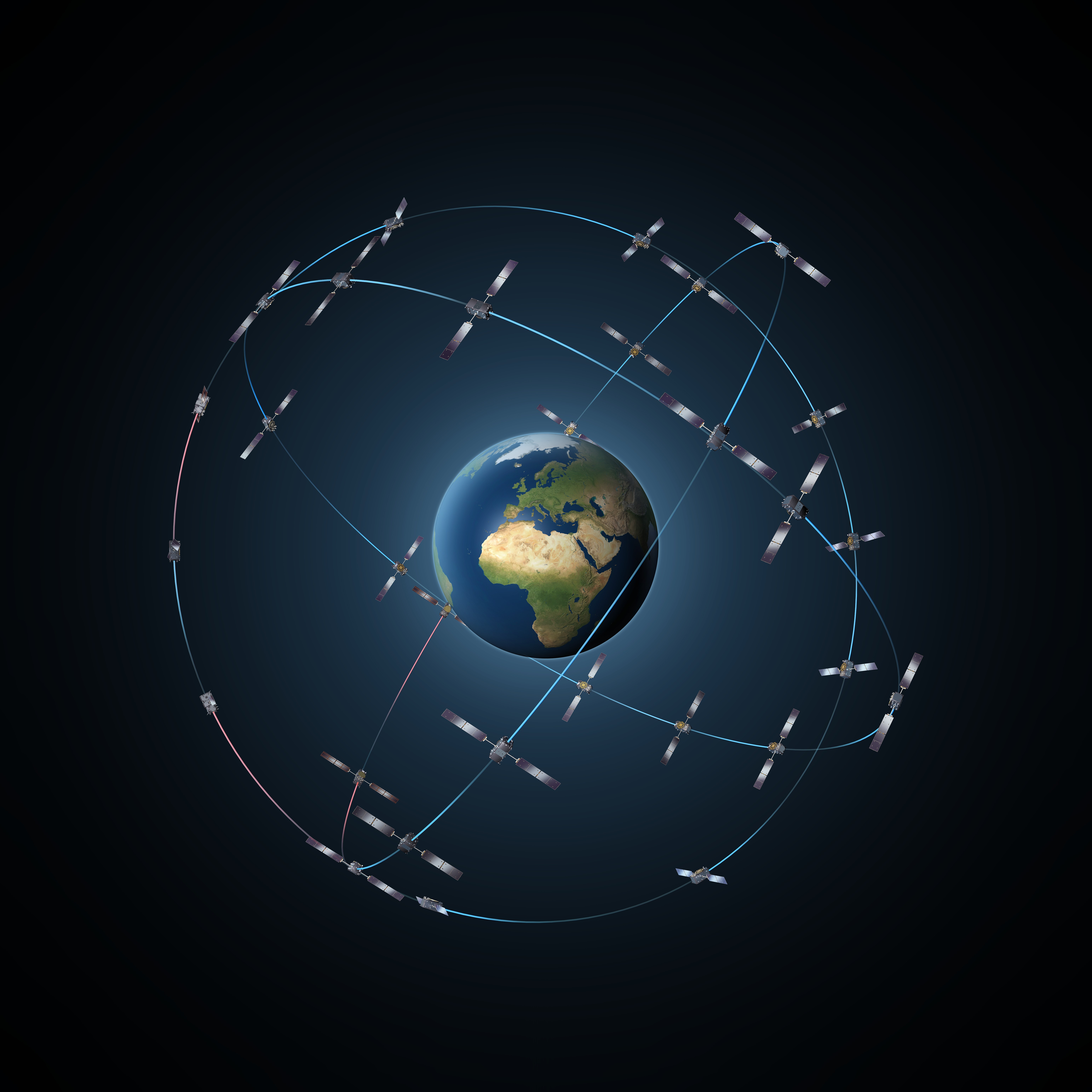
Galileo uses a Walker 24/3/1 constellation: 24 operational satellites distributed across 3 orbital planes (A, B, C), each separated by 120° in RAAN. Each plane contains 8 evenly-spaced satellites (45° apart), with a phasing factor of 1 — meaning satellites in adjacent planes are offset by 40°. This ensures that every point on Earth always has at least 4 satellites above the horizon, the minimum needed for a 3D position fix. Six additional satellites serve as in-orbit spares, bringing the total to 30.
Orbit Definition
Each orbit is described by six numbers called Keplerian elements. In everyday terms: how big the orbit is (semi-major axis \(a\)), how circular or oval it is (eccentricity \(e\)), how tilted relative to the equator (inclination \(i\)), which direction the tilt faces (RAAN \(\Omega\)), where the closest point is (argument of perigee \(\omega\)), and where the satellite starts (true anomaly \(\nu\)).
Earth's Shape Matters
Earth is slightly flattened at the poles — it bulges at the equator. This bulge (known as "J2" in geodesy) gradually rotates the orientation of every orbit. Without modelling this effect, satellite positions would drift by tens of kilometres per day compared to reality. The simulator includes J2 as an additional gravitational pull that slightly tugs satellites toward the equatorial plane.
Deep dive: J2 perturbation mathematics
The J2 perturbation adds an acceleration term to the two-body equations of motion:
\[ \mathbf{a}_{J_2} = -\frac{3}{2}\,J_2\,\mu\,\frac{R_E^2}{r^4} \left[\left(1 - 5\frac{z^2}{r^2}\right)\hat{\mathbf{r}} + 2\frac{z}{r}\,\hat{\mathbf{z}}\right] \]where \(J_2 = 1.08263 \times 10^{-3}\) is the oblateness coefficient, \(\mu = 3.986 \times 10^{14}\;\text{m}^3/\text{s}^2\) is Earth's gravitational parameter, and \(R_E = 6{,}371\;\text{km}\) is the mean Earth radius. The term \((z/r)^2\) represents the sine of the satellite's geocentric latitude squared, which is why the perturbation depends on how far the satellite is from the equatorial plane.
For Galileo-type MEO orbits (~23,222 km altitude, 56° inclination), this produces RAAN drift of approximately \(0.04°/\text{day}\) — small but critical for maintaining constellation geometry over weeks and months.
Worked example: Consider GSAT0101 at altitude \(h = 23{,}222\;\text{km}\), so \(r = R_E + h = 29{,}593\;\text{km}\). The satellite is at latitude 30°N, so \(z = r \sin(30°) = 14{,}797\;\text{km}\) and \(z^2/r^2 = 0.25\). Plugging in:
\[ a_{J_2} = \frac{3}{2} \times 1.083 \times 10^{-3} \times \frac{3.986 \times 10^{14} \times (6.371 \times 10^6)^2} {(2.959 \times 10^7)^4} \]The prefactor evaluates to approximately \(9.1 \times 10^{-5}\;\text{m/s}^2\). The radial component is scaled by \((1 - 5 \times 0.25) = -0.25\) and the z-component by \(2 \times 0.5 = 1.0\). This tiny acceleration — about one hundred-thousandth of surface gravity — accumulates over hours to shift the orbital plane by \(\sim 0.04°\) per day. After one month the RAAN has drifted \(\sim 1.2°\), and after a year \(\sim 15°\) — enough to visibly rearrange the constellation if not accounted for.
Beyond J2: The Full Force Model
Real spacecraft are subject to more than just Earth's gravity. The simulator includes a comprehensive force model that sums all significant perturbations at each integration step:
- Zonal gravity harmonics (J2–J6) — Earth's oblateness and slight pear-shape cause the orbit to slowly drift. J2 is the dominant effect, but higher-order terms add small corrections
- Atmospheric drag — at low altitudes (<1,000 km), the thin residual atmosphere slows satellites down, gradually lowering their orbit. The drag varies with solar activity — a more active Sun heats and expands the upper atmosphere
- Solar radiation pressure — sunlight itself pushes on the satellite. The force is tiny but constant (except during eclipse), and over months it shifts the orbit measurably
- Sun and Moon gravity — the gravitational pull of the Sun and Moon tugs on satellites, causing kilometre-level position shifts over weeks if not modelled
Stepping Forward in Time
The simulator advances each satellite's position and velocity using a numerical method called RK4 (4th-order Runge-Kutta). Think of it as taking small time steps and carefully computing where all forces will have moved the satellite by the next step. RK4 is widely used in physics simulations because it provides a good balance of accuracy and computational cost.
Deep dive: RK4 integration and coordinate frames
The integrator advances a 6-element state vector \(\mathbf{y} = [x, y, z, v_x, v_y, v_z]\) with a fixed time step \(\Delta t\). At each of the four RK4 sub-steps, the total acceleration is computed by summing zonal gravity (J2–J6), atmospheric drag, solar radiation pressure, and Sun/Moon third-body perturbations. The sub-satellite point is derived by transforming the resulting ECI position to geodetic coordinates.
Three coordinate frames are used throughout:
- ECI (Earth-Centred Inertial) — a non-rotating frame anchored to the stars, used for orbit propagation
- ECEF (Earth-Centred Earth-Fixed) — rotates with the Earth, used for GPS and ground geometry
- Geodetic (latitude, longitude, altitude) — the familiar map coordinates, used for display
ECI↔ECEF conversion applies Earth's rotation rate \(\omega_E = 7.2921 \times 10^{-5}\;\text{rad/s}\) as a rotation about the z-axis. ECEF↔geodetic uses an iterative method on the WGS-84 ellipsoid (\(a = 6{,}378{,}137\;\text{m}\), \(f = 1/298.257\)), which accounts for Earth's oblate shape when computing latitude and altitude above the surface.
Worked example — one RK4 step: GSAT0101 is at position \(\mathbf{r} = (25{,}000,\; 15{,}000,\; 5{,}000)\;\text{km}\) with velocity \(\mathbf{v} = (-1.2,\; 2.8,\; 1.5)\;\text{km/s}\) and we step by \(\Delta t = 10\;\text{s}\). The integrator evaluates four sub-steps:
- k1: Compute acceleration at the current state. Gravity gives \(\mathbf{a} = -\mu/r^3 \cdot \mathbf{r}\) where \(r = 29{,}580\;\text{km}\), so \(|\mathbf{a}| \approx 0.46\;\text{m/s}^2\) (directed toward Earth). Add J2 correction (~\(10^{-5}\;\text{m/s}^2\)).
- k2: Advance state by \(\frac{1}{2}\Delta t\) using k1, recompute acceleration at the midpoint. Position shifts by ~\(14\;\text{m}\), velocity by ~\(2.3\;\text{mm/s}\).
- k3: Advance from original state by \(\frac{1}{2}\Delta t\) using k2, recompute. Nearly identical to k2 for this short step.
- k4: Advance by full \(\Delta t\) using k3, recompute at the endpoint.
The weighted average \(\frac{1}{6}(k_1 + 2k_2 + 2k_3 + k_4)\) gives the final update. After one step the satellite has moved ~29 km along its orbit (about 0.1% of a full revolution), and the accumulated position error from the numerical integration is less than \(10^{-6}\;\text{m}\) — negligible compared to the J2 perturbation effects we're modelling.
03. GPS Receiver Simulation
The web interface includes a simulated GPS receiver. It uses your real location (from your browser) and the simulated constellation overhead to compute a navigation fix — exactly as a real GPS receiver would. The result includes realistic errors from atmosphere, signal reflections, and satellite geometry.
How GPS Works (In Brief)
A GPS receiver measures how long radio signals take to travel from each visible satellite. Multiplying by the speed of light gives a distance (called a pseudorange) to each satellite. With distances to at least four satellites whose positions are known, the receiver can compute its own position. The fourth satellite is needed because the receiver's clock isn't perfectly synchronised with the satellites' atomic clocks.
Error Sources
In the real world, pseudoranges are never perfect. The signal passes through the atmosphere (which slows it down), bounces off buildings and terrain (multipath), and the satellite and receiver clocks have small errors. The simulator models all of these:
| Error source | What causes it | How much |
|---|---|---|
| Ionosphere | Charged particles in the upper atmosphere slow the signal; modelled using the Klobuchar algorithm with elevation-dependent obliquity factor | 5–50 m |
| Troposphere | The lower atmosphere (air, moisture) also slows the signal; worse near the horizon | 2.6–25 m |
| Multipath | Signal reflects off ground/buildings before reaching antenna; worse at low elevation | 0.1–1.5 m |
| Satellite clock | Allan variance noise model (white frequency + random walk) propagated in the RINEX af0/af1 parameters. Three clock types supported: PHM (~100 ns/day), RAFS (~300 ns/day), OCXO (~10 μs/day) | \(\sigma = 0.5\;\text{m}\) |
| Broadcast ephemeris | Satellite positions are computed from broadcast Keplerian elements rather than true state. The prediction degrades as the orbit drifts from the snapshot due to unmodelled perturbations (J2+, drag, SRP, third-body) | 1–5 m |
| OD&TS | Ground-segment orbit determination and time synchronisation prediction error. Independent of broadcast ephemeris drift | \(\sigma = 0.65\;\text{m}\) |
| Receiver noise | Thermal noise in the receiver electronics. Dual-frequency receivers have ~1.4× higher noise from combining two signals | \(\sigma = 2.0\;\text{m}\) (single) / \(2.8\;\text{m}\) (dual) |
Deep dive: pseudorange equation
For each satellite above the elevation mask (default 5°), the simulated pseudorange is:
\[ \rho = R_{\text{true}} + c\,\delta t_{rx} + I(\text{el},\,t) + T(\text{el}) + M(\text{el}) + \varepsilon_{\text{clk}} + \varepsilon_{\text{rx}} \]where:
| Term | Description | Value / model |
|---|---|---|
| \(R_{\text{true}}\) | Geometric range: Euclidean distance from receiver to satellite in ECEF | ~25,000–29,000 km for Galileo MEO |
| \(c\,\delta t_{rx}\) | Receiver clock bias, solved as the 4th unknown in the navigation solution | 1,000 m (simulated constant) |
| \(I(\text{el},\,t)\) | Ionospheric delay — see Atmospheric Models | \(F(\text{el}) \cdot I_{\text{zenith}}(t)\) |
| \(T(\text{el})\) | Tropospheric delay — Saastamoinen mapping | \((2.3 + 0.3)\,/\,\sin(\text{el} + \text{corr})\) |
| \(M(\text{el})\) | Multipath: bias \(\cdot\, e^{-\text{el}/20}\) + noise \(\cdot\, \mathcal{N}(0,1) \cdot e^{-\text{el}/10}\) | Exponential decay with elevation |
| \(\varepsilon_{\text{clk}}\) | Satellite clock residual | \(\mathcal{N}(0,\; 0.5^2)\) |
| \(\varepsilon_{\text{rx}}\) | Receiver thermal noise | \(\mathcal{N}(0,\; 2.0^2)\) |
Worked example: A satellite at 25° elevation is 23,500 km away (geometric range). The receiver clock is biased by 1,000 m equivalent. It's 14:00 local time (peak ionosphere). Plugging in:
| Term | Calculation | Value |
|---|---|---|
| \(R_{\text{true}}\) | Geometric distance | 23,500,000 m |
| \(c\,\delta t_{rx}\) | Clock bias | +1,000.0 m |
| \(I\) | \(F(25°) \approx 1.5\) × \(I_{\text{zenith}} = 15\;\text{m}\) | +22.5 m |
| \(T\) | \(2.6\,/\,\sin(25° + 7.6°/(25°+3.3°)) \approx 2.6/0.46\) | +5.7 m |
| \(M\) | \(1.0 \cdot e^{-25/20} + 0.5 \cdot (+0.8) \cdot e^{-25/10}\) | +0.32 m |
| \(\varepsilon_{\text{clk}}\) | Random draw \(\mathcal{N}(0,\,0.25)\) | +0.3 m |
| \(\varepsilon_{\text{rx}}\) | Random draw \(\mathcal{N}(0,\,4.0)\) | −1.1 m |
| Total \(\rho\) | 23,501,027.7 m |
The true distance is 23,500 km, but the measured pseudorange is 23,501,028 m — off by 1,028 m, dominated by the receiver clock bias (which the solver removes). The remaining ~28 m of atmospheric and noise errors is what limits position accuracy.
04. Atmospheric Error Models
The atmosphere is the largest source of GPS error. The simulator models two distinct layers and one ground-level effect.
Ionospheric Delay
The ionosphere (60–1,000 km altitude) contains electrically charged particles created by solar radiation. These particles slow GPS signals, adding 5–50 m of apparent extra distance. The delay depends on two things:
- Satellite elevation — a signal from a satellite near the horizon travels through much more ionosphere than one from directly overhead (up to 3× more)
- Time of day — solar UV creates more charged particles during daytime, peaking around 14:00 local time. Night-time delays are roughly one-third of daytime values
Deep dive: ionospheric model equations
The model is based on the Klobuchar broadcast ionosphere correction used in GPS. It has two components:
Obliquity factor — converts zenith (overhead) delay to slant delay for the actual satellite elevation. This is a thin-shell approximation treating the ionosphere as a layer at ~350 km altitude:
\[ F(\text{el}) = 1 + 16 \left(0.53 - \frac{\text{el}}{180}\right)^3 \]At 5° elevation, \(F \approx 3.0\) (three times the overhead delay). At 90° (zenith), \(F \approx 1.0\). The cubic form approximates the secant of the zenith angle at the ionospheric pierce point.
Diurnal variation — the zenith delay follows a half-cosine during daytime and is constant at night:
\[ I_{\text{zenith}}(t) = I_{\min} + (I_{\max} - I_{\min}) \cdot \max\!\left(0,\; \cos\frac{2\pi(t - 50400)}{86400}\right) \]where \(I_{\min} = 5\;\text{m}\) (night-time floor), \(I_{\max} = 15\;\text{m}\) (daytime peak), and \(50{,}400\;\text{s} = \text{14:00 UTC}\). The \(\max(0, \ldots)\) clamps the delay to the minimum during night-time hours when the cosine goes negative. The final ionospheric delay is \(F(\text{el}) \cdot I_{\text{zenith}}(t)\).
Worked example: A satellite at 10° elevation, observed at 14:00 local time (peak ionosphere).
Step 1 — Obliquity factor:
\[ F(10°) = 1 + 16\,(0.53 - 10/180)^3 = 1 + 16 \times 0.474^3 = 1 + 16 \times 0.107 = 2.71 \]Step 2 — Zenith delay at 14:00 (peak): \(t = 50{,}400\;\text{s}\), so the cosine argument is zero and \(\cos(0) = 1\):
\[ I_{\text{zenith}} = 5 + (15 - 5) \times \max(0,\;1) = 15\;\text{m} \]Step 3 — Total ionospheric delay:
\[ I = F \times I_{\text{zenith}} = 2.71 \times 15 = 40.7\;\text{m} \]Now compare: the same satellite at 14:00 but at 60° elevation would give \(F(60°) = 1 + 16 \times 0.197^3 = 1.12\) and \(I = 1.12 \times 15 = 16.8\;\text{m}\). At 10° elevation but 02:00 at night, the zenith delay drops to 5 m (the cosine is negative, clamped to zero) and \(I = 2.71 \times 5 = 13.6\;\text{m}\). This shows why low-elevation daytime measurements are the noisiest.
Tropospheric Delay
The troposphere (0–12 km) is the air you breathe. It delays GPS signals by about 2.3 m when looking straight up (from the "dry" air) plus another 0.3 m from water vapour. When a satellite is near the horizon, the signal travels through far more air, and the delay can exceed 25 m.
Deep dive: Saastamoinen tropospheric mapping
The zenith delay is split into dry (hydrostatic) and wet components, then mapped to slant delay using a modified sine function:
\[ T(\text{el}) = \frac{T_{\text{dry}} + T_{\text{wet}}} {\sin\!\left(\text{el} + \dfrac{7.6°}{\text{el} + 3.3°}\right)} \]The correction term \(7.6/(\text{el} + 3.3)\) in the argument prevents the function from going to infinity at zero elevation (a pure \(1/\sin(\text{el})\) would). This modified mapping matches full ray-tracing results to within a few percent for elevations above 5°.
Worked example at 10° elevation:
Step 1 — Compute the correction term: \(7.6° / (10° + 3.3°) = 7.6 / 13.3 = 0.571°\)
Step 2 — Modified sine: \(\sin(10° + 0.571°) = \sin(10.571°) = 0.1835\)
Step 3 — Tropospheric delay:
\[ T(10°) = \frac{2.3 + 0.3}{0.1835} = \frac{2.6}{0.1835} = 14.2\;\text{m} \]For comparison, step through two more elevations:
| Elevation | Correction | sin(el + corr) | T (metres) |
|---|---|---|---|
| 5° | \(7.6/8.3 = 0.916°\) | \(\sin(5.916°) = 0.1031\) | \(2.6 / 0.103 = 25.2\) |
| 10° | \(7.6/13.3 = 0.571°\) | \(\sin(10.571°) = 0.1835\) | \(2.6 / 0.184 = 14.2\) |
| 30° | \(7.6/33.3 = 0.228°\) | \(\sin(30.228°) = 0.5038\) | \(2.6 / 0.504 = 5.2\) |
| 90° | \(7.6/93.3 = 0.081°\) | \(\sin(90.081°) \approx 1.0\) | \(2.6 / 1.0 = 2.6\) |
The delay nearly doubles from 14 m to 25 m between 10° and 5° — this rapid increase at low elevations is one reason GPS receivers use a minimum elevation mask.
Multipath
Multipath occurs when a GPS signal bounces off the ground, buildings, or other surfaces before reaching the antenna. The reflected signal arrives slightly later than the direct signal, corrupting the range measurement. Multipath is worst for low-elevation satellites (more ground reflections) and is modelled as an exponentially decaying bias plus random noise:
- Systematic bias — up to 1.0 m at the horizon, decaying to near zero at high elevations
- Random scatter — up to 0.5 m standard deviation at low elevations, negligible above 45°
Deep dive: multipath model
The multipath error for a satellite at elevation \(\text{el}\) (degrees) is:
\[ M(\text{el}) = 1.0 \cdot e^{-\text{el}/20} + 0.5 \cdot \mathcal{N}(0,1) \cdot e^{-\text{el}/10} \]The first term is a deterministic bias that models the systematic effect of ground-plane reflections. The second is zero-mean Gaussian noise whose standard deviation decays faster with elevation (\(e^{-\text{el}/10}\) vs \(e^{-\text{el}/20}\)) because the random multipath environment becomes less significant as the satellite rises above surrounding obstacles.
Worked example at 5° elevation:
Bias term: \(1.0 \times e^{-5/20} = 1.0 \times e^{-0.25} = 1.0 \times 0.779 = 0.78\;\text{m}\)
Noise standard deviation: \(0.5 \times e^{-5/10} = 0.5 \times e^{-0.5} = 0.5 \times 0.607 = 0.30\;\text{m}\)
So if the random draw is \(\mathcal{N}(0,1) = +1.2\), the total multipath error is \(0.78 + 0.30 \times 1.2 = 1.14\;\text{m}\). This satellite near the horizon might be receiving signals bouncing off a building before reaching the antenna.
Summary across elevations:
| Elevation | Bias (m) | Noise \(\sigma\) (m) | Typical total |
|---|---|---|---|
| 5° | 0.78 | 0.30 | ~1.1 m |
| 30° | 0.22 | 0.02 | ~0.2 m |
| 60° | 0.05 | ~0 | ~0.05 m |
| 90° | 0.01 | ~0 | ~0.01 m |
A satellite directly overhead has virtually no multipath because there are no reflecting surfaces above the antenna. A satellite at 5° can easily add a metre of error — comparable to the tropospheric delay.
05. Navigation Solver
Given pseudorange measurements to several satellites, the solver figures out where the receiver is. It needs to solve for four unknowns: three position coordinates (X, Y, Z) and the receiver clock error. This is an over-determined system when more than four satellites are visible (which is typical), so the solver finds the best-fit solution.
Iterative Approach
The solver starts with a rough guess and refines it repeatedly. At each step, it computes "if I were at this guess position, how far off would my predicted ranges be from the measured ranges?" and adjusts accordingly. This converges to the correct position within 4–6 iterations, typically in under a millisecond.
Elevation Weighting
Not all satellites contribute equally to a good fix. Low-elevation satellites have noisier measurements (more atmosphere, more multipath), so the solver gives less weight to their measurements and more weight to high-elevation satellites. This is standard practice in real GPS receivers.
Deep dive: Gauss-Newton weighted least squares
The solver uses the Gauss-Newton method on the nonlinear pseudorange equations. The state vector is \(\mathbf{x} = [X,\,Y,\,Z,\,c\,\delta t]\) in ECEF coordinates. At each iteration, the design matrix row for satellite \(i\) is:
\[ H_i = \begin{bmatrix} \dfrac{\Delta x_i}{r_i} & \dfrac{\Delta y_i}{r_i} & \dfrac{\Delta z_i}{r_i} & 1 \end{bmatrix} \]where \(\Delta x, \Delta y, \Delta z\) are the components of the vector from the current position estimate to satellite \(i\), and \(r\) is its magnitude. These are the unit line-of-sight direction cosines plus a column of ones for the clock.
The residual for each satellite is \(r_i = \rho_{\text{meas}} - r_{\text{pred}} - c\,\delta t\). The state update is:
\[ \delta\mathbf{x} = \left(H^\top W H\right)^{-1} H^\top W\,\mathbf{r} \]where \(W = \text{diag}(\sin \text{el}_i)\) is the elevation-dependent weight matrix. The \(\sin\) weighting downweights low-elevation measurements (which have more atmospheric error) while preserving enough geometric contribution from them for vertical positioning. Convergence is declared when the position shift \(|\delta\mathbf{x}|\) falls below \(10^{-4}\;\text{m}\).
The 4×4 normal equations are solved by Gaussian elimination with partial pivoting, which is efficient for this small system and avoids the overhead of a general linear algebra library.
Worked example: Suppose we have 6 Galileo satellites in view from Munich (48.1°N, 11.6°E). The receiver starts with an initial guess 100 km off from the true position and a clock bias of zero.
Iteration 1: The solver computes the predicted range to each satellite from its guess position and compares to the measured pseudoranges. The residuals are large (~100 km). The \(H\) matrix rows are the unit direction vectors from guess to each satellite. Solving \(\delta\mathbf{x} = (H^\top W H)^{-1} H^\top W \mathbf{r}\) yields a correction of about 95 km toward the true position, plus a clock bias estimate of ~980 m.
Iteration 2: From the new position (now ~5 km off), residuals drop to ~5 km. The direction cosines change slightly. The correction is ~4.9 km.
Iteration 3: Residuals are ~100 m. Correction: 99.8 m.
Iteration 4: Residuals are ~0.3 m. Correction: 0.28 m.
Iteration 5: Correction < \(10^{-4}\;\text{m}\) — converged. The final position is within ~15 m of truth (limited by measurement noise, not the solver). Total computation time: < 0.1 ms. The \(\sin\) weighting means that a satellite at 60° elevation (weight 0.87) contributes 3.3× more to the solution than one at 15° (weight 0.26).
Dilution of Precision (DOP)
Even with perfect range measurements, the position accuracy depends on satellite geometry. If all visible satellites are clustered in one part of the sky, the position fix is poor (high DOP). If they're spread evenly, the fix is good (low DOP). The simulator reports four DOP values:
| Metric | Meaning | Good value |
|---|---|---|
| HDOP | Horizontal accuracy factor — multiply by UERE for horizontal error estimate | < 2 |
| VDOP | Vertical accuracy factor — usually worse than HDOP because all satellites are above you | < 3 |
| PDOP | 3D position accuracy factor | < 3 |
| GDOP | Overall geometry factor including clock uncertainty | < 5 |
As a rule of thumb: position error ≈ UERE × DOP. With UERE ≈ 10 m and HDOP ≈ 1.5, expect horizontal errors around 15 m. Vertical errors are typically 1.5–3× larger.
Deep dive: DOP computation from covariance matrix
After the solver converges, the covariance matrix of the solution is:
\[ Q = \left(H^\top W H\right)^{-1} \]This 4×4 matrix describes the uncertainty of \([X,\,Y,\,Z,\,\text{clock}]\) in ECEF coordinates. To extract meaningful horizontal and vertical DOP, the 3×3 position block is rotated into a local East-North-Up (ENU) frame at the solved position using the standard ECEF→ENU rotation matrix \(R\):
\[ Q_{\text{ENU}} = R\,Q_{\text{XYZ}}\,R^\top \]The DOP values are then:
\[ \text{HDOP} = \sqrt{Q_{EE} + Q_{NN}} \qquad \text{VDOP} = \sqrt{Q_{UU}} \qquad \text{PDOP} = \sqrt{Q_{EE} + Q_{NN} + Q_{UU}} \qquad \text{GDOP} = \sqrt{Q_{EE} + Q_{NN} + Q_{UU} + Q_{\text{clk}}} \]The ENU rotation is necessary because ECEF X, Y, Z do not correspond to horizontal and vertical at an arbitrary receiver location. Without it, HDOP and VDOP would only be correct at the north pole.
Note that DOP depends only on geometry (the \(H\) matrix), not on measurement quality. Two receivers at the same location seeing the same satellites will have identical DOP values regardless of their noise characteristics. DOP becomes a pure multiplier on whatever range error budget exists.
Worked example: Six Galileo satellites are visible from Munich. After the solver converges and the covariance is rotated to ENU, the diagonal is:
\[ Q_{EE} = 0.82 \qquad Q_{NN} = 0.94 \qquad Q_{UU} = 2.15 \qquad Q_{\text{clk}} = 1.40 \]Computing the DOP values:
| DOP | Formula | Value | Interpretation |
|---|---|---|---|
| HDOP | \(\sqrt{0.82 + 0.94}\) | 1.33 | Excellent — satellites spread well in azimuth |
| VDOP | \(\sqrt{2.15}\) | 1.47 | Good — but worse than horizontal because all sats are above |
| PDOP | \(\sqrt{0.82 + 0.94 + 2.15}\) | 1.98 | Good 3D geometry |
| GDOP | \(\sqrt{0.82 + 0.94 + 2.15 + 1.40}\) | 2.30 | Good overall |
With a UERE of ~10 m, the expected horizontal error is \(10 \times 1.33 \approx 13\;\text{m}\) and vertical error is \(10 \times 1.47 \approx 15\;\text{m}\). If one satellite drops below the horizon and the remaining five are clustered in the north, HDOP might jump to 3.5, degrading horizontal accuracy to ~35 m — the same measurement noise, but worse geometry.
06. Spacecraft Subsystems
Each simulated satellite models six core subsystems. These interact realistically — for example, entering Earth's shadow cuts solar power, which drains the battery, which may trigger safe mode, which changes the attitude control mode.
Electrical Power System (EPS)
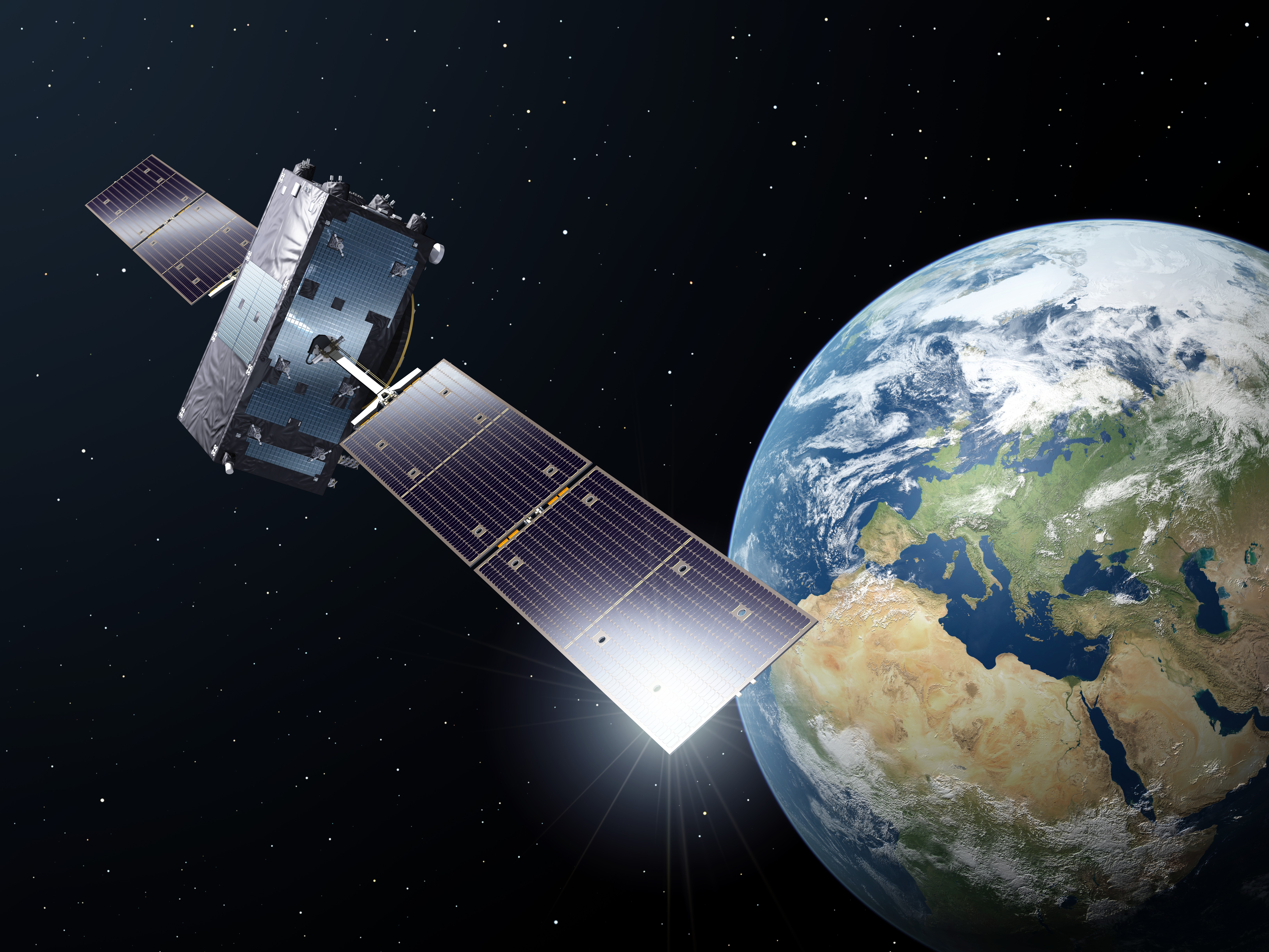
Each Galileo satellite carries two solar wings generating approximately 1,500 W at beginning of life, with lithium-ion batteries providing 3,240 Wh of storage on a regulated 50 V bus. Solar power depends on illumination fraction and the angle between the panels and the Sun. Eclipse transitions use a penumbra model that computes the fraction of the Sun's disk obscured by Earth, giving a smooth 4–10 second transition rather than an abrupt on/off switch. The battery charges when solar power exceeds the electrical load and discharges otherwise. If the state of charge (SOC) drops below 20%, the satellite autonomously enters safe mode — shedding non-essential loads to protect the battery.
The total electrical load is approximately 900 W during nominal operations, dominated by the navigation payload and atomic clocks. Each satellite carries four atomic clocks for redundancy — two Passive Hydrogen Masers (PHM, stability \(\leq 1 \times 10^{-14}\) over 10,000 s) and two Rubidium Atomic Frequency Standards (RAFS, stability \(\leq 5 \times 10^{-13}\) over 100 s). The simulation models one active clock per satellite; the clock type determines the Allan variance noise characteristics.
Solar panels degrade slowly over time from radiation and thermal cycling, reducing maximum power over the mission lifetime. Battery efficiency varies with charge level and temperature, and the battery slowly self-discharges when not in use — faster when hot.
Attitude Determination and Control (ADCS)
Controls the satellite's orientation using three reaction wheels (spinning flywheels that can rotate the spacecraft by changing their speed) and magnetic torquers (electromagnets that push against Earth's magnetic field). Pointing modes include sun-pointing (for maximum solar power), Earth-pointing (for communications), and target-pointing.
When reaction wheels accumulate too much momentum, the system automatically "desaturates" them using the magnetic torquers. This works better at lower altitudes where Earth's magnetic field is stronger. As wheels approach saturation, the satellite's ability to turn quickly degrades.
Thermal Control
The thermal model tracks temperatures of key components: onboard computer, battery, payload, structure, and radiator panels. Heat from sunlight is absorbed on the sun-facing side, while radiator panels on the opposite side radiate heat into space. Heat also flows between components through conduction. Heaters keep components warm during eclipse. If any component gets too hot, the fault management system sheds loads to protect the spacecraft.
Deep dive: thermal radiation
Each radiator panel's heat rejection follows:
\[ P_{\text{rad}} = \varepsilon\,\sigma\,A\,T^4 \]where \(\varepsilon\) is the surface emissivity, \(\sigma = 5.67 \times 10^{-8}\;\text{W/m}^2\text{K}^4\) is the Stefan-Boltzmann constant, \(A\) is the radiator area, and \(T\) is the surface temperature in Kelvin. The \(T^4\) dependence means that small temperature changes produce large changes in radiated power, creating a natural self-regulating effect.
Worked example: A Galileo satellite's radiator panel has emissivity \(\varepsilon = 0.85\) and area \(A = 2.0\;\text{m}^2\). Compare the radiated power at two temperatures:
At 300 K (27°C, nominal operations):
\[ P = 0.85 \times 5.67 \times 10^{-8} \times 2.0 \times 300^4 = 0.85 \times 5.67 \times 10^{-8} \times 2.0 \times 8.1 \times 10^9 = 780\;\text{W} \]At 340 K (67°C, thermal alarm threshold):
\[ P = 0.85 \times 5.67 \times 10^{-8} \times 2.0 \times 340^4 = 0.85 \times 5.67 \times 10^{-8} \times 2.0 \times 1.336 \times 10^{10} = 1{,}286\;\text{W} \]A 13% temperature increase (300→340 K) produces a 65% increase in radiated power (780→1,286 W). This is the \(T^4\) self-regulating effect: when a component gets hotter, it sheds heat much faster, naturally resisting runaway temperature increases. This is also why spacecraft in eclipse cool rapidly — the radiators keep dumping heat even after solar input drops to zero.
Communications
A ground station can communicate with a satellite only when it is above the station's horizon. Inter-satellite links (ISL) connect satellites that have line-of-sight to each other, enabling data relay across the constellation. The laser links require precise pointing — a satellite in safe mode cannot maintain a link, and manoeuvring reduces signal quality.
The ISL topology is visualised both on the 3D globe (faint green arcs) and on
the Mercator map (green lines). The dedicated ISL topology graph arranges
satellites by orbital plane and shows link status with range on hover. Operators
can ping peer satellites over the ISL mesh to measure round-trip
time, or run traceroute to find the shortest delay path using
Dijkstra’s algorithm with propagation delay as the edge weight.
Contact history is tracked server-side per ground station. Each completed pass is recorded with AOS/LOS timestamps, maximum elevation, and duration. Shell command history is also persisted on the server (up to 200 entries per station), so terminal logs survive page navigation.
Propulsion
A thruster system provides delta-V (velocity changes) for orbit maintenance. Fuel mass is tracked and decremented during burns. Thruster faults can be injected for testing: a stuck-open thruster leaks fuel uncontrollably, while a stuck-closed thruster reduces available thrust.
Deep dive: Tsiolkovsky rocket equation
The achievable velocity change from a burn is governed by the rocket equation:
\[ \Delta v = I_{sp}\,g_0\,\ln\frac{m_0}{m_f} \]where \(I_{sp}\) is the specific impulse (a measure of thruster efficiency), \(g_0 = 9.80665\;\text{m/s}^2\), \(m_0\) is the initial mass, and \(m_f\) is the final mass after fuel is expended. The logarithmic relationship means that doubling the fuel doesn't double the delta-V — there are diminishing returns as the spacecraft gets heavier.
Worked example: A Galileo satellite has dry mass 680 kg, fuel mass 80 kg (total \(m_0 = 760\;\text{kg}\)), and thrusters with \(I_{sp} = 285\;\text{s}\) (typical bipropellant). What delta-V is available?
\[ \Delta v = 285 \times 9.807 \times \ln\frac{760}{680} = 2{,}795 \times \ln(1.118) = 2{,}795 \times 0.1112 = 311\;\text{m/s} \]This 311 m/s budget must cover the satellite's entire 12-year mission: orbit insertion correction, periodic station-keeping manoeuvres, and end-of-life de-orbit. A typical station-keeping burn uses ~0.5 m/s, meaning the satellite can perform roughly 600 such manoeuvres.
Now see the diminishing returns: if we doubled the fuel to 160 kg (\(m_0 = 840\;\text{kg}\)), the delta-V becomes \(2{,}795 \times \ln(840/680) = 2{,}795 \times 0.211 = 590\;\text{m/s}\) — only 1.9× more delta-V for 2× the fuel, because the heavier fuel load makes the spacecraft harder to accelerate.
Radiation Environment
Satellites in MEO pass through the Van Allen radiation belts — zones of trapped charged particles held by Earth's magnetic field. Galileo satellites at 23,222 km sit near the peak of the outer electron belt, so they receive a significant radiation dose over their lifetime. The simulator models this radiation and its effect on electronics: high-energy particles occasionally cause random bit flips (Single Event Upsets) in onboard memory and processors.
Space Weather
The Sun's activity affects the space environment. The simulator tracks two indicators: the Kp geomagnetic index (how disturbed Earth's magnetic field is) and the F10.7 solar radio flux (how active the Sun is). Geomagnetic storms arrive periodically, intensifying the radiation belts and increasing the rate of electronics upsets. Solar activity also affects how much the upper atmosphere drags on low-orbit satellites.
Fuel Slosh
When a thruster burn ends, liquid propellant in the tank sloshes back and forth, briefly disturbing the satellite's orientation. The effect is stronger with fuller tanks and is visible in the reaction wheel telemetry immediately after burns.
Leap Second Handling
GNSS systems must keep precise track of time. The simulation maintains the offset between atomic time (TAI) and everyday time (UTC), which changes whenever a leap second is added. This offset is needed to correctly convert between GPS time, satellite time, and the UTC time shown to users.
back to top07. Ground Segment

Ground Station Contacts
A ground station can communicate with a satellite only when the satellite is above the local horizon — just as you can only see an aeroplane when it's above the surrounding terrain. The simulator computes this by checking the elevation angle from each station to each satellite in real time. The elevation angle is the angle between the horizon and the line to the satellite: 0° means on the horizon, 90° means directly overhead.
Deep dive: elevation angle computation
The elevation angle is computed from the dot product of two vectors in ECEF coordinates: the station-to-satellite vector and the station's local vertical (the outward normal to the WGS-84 ellipsoid at the station's position).
For a station at ECEF position \(\mathbf{s}\) and satellite at \(\mathbf{p}\), the elevation is:
\[ \text{el} = \arcsin\frac{(\mathbf{p} - \mathbf{s}) \cdot \hat{\mathbf{n}}} {|\mathbf{p} - \mathbf{s}|} \]where \(\hat{\mathbf{n}}\) is the unit normal to the ellipsoid at the station. For a spherical Earth approximation, \(\hat{\mathbf{n}} = \mathbf{s}/|\mathbf{s}|\). A contact exists when \(\text{el}\) exceeds the station's minimum elevation mask (typically 5–10° to account for terrain and atmospheric effects near the horizon).
Worked example: The Fucino ground station (Italy, 42.0°N, 13.6°E) wants to communicate with GSAT0101. Using a spherical Earth approximation:
Step 1: Convert Fucino to ECEF. \(\mathbf{s} = R_E [\cos(42°)\cos(13.6°),\;\cos(42°)\sin(13.6°),\;\sin(42°)]\) \(= [4{,}589,\; 1{,}113,\; 4{,}262]\;\text{km}\)
Step 2: Suppose GSAT0101 is at ECEF position \(\mathbf{p} = [18{,}000,\; 10{,}000,\; 20{,}000]\;\text{km}\). The station-to-satellite vector is \(\mathbf{d} = \mathbf{p} - \mathbf{s} = [13{,}411,\; 8{,}887,\; 15{,}738]\;\text{km}\), with magnitude \(|\mathbf{d}| = 22{,}660\;\text{km}\).
Step 3: The local vertical at Fucino is \(\hat{\mathbf{n}} = \mathbf{s}/|\mathbf{s}| = [0.719,\; 0.175,\; 0.668]\). The dot product is: \(\mathbf{d} \cdot \hat{\mathbf{n}} = 13{,}411 \times 0.719 + 8{,}887 \times 0.175 + 15{,}738 \times 0.668 = 21{,}689\;\text{km}\)
Step 4: Elevation angle:
\[ \text{el} = \arcsin\frac{21{,}689}{22{,}660} = \arcsin(0.957) = 73.2° \]At 73° elevation, this is an excellent pass — nearly overhead. The link quality will be high and atmospheric errors minimal. If the station's elevation mask is 5°, this satellite is well above it. When the satellite moves and the elevation drops below 5°, a Loss of Signal (LOS) event is logged.
GPS Receiver Integration
The browser-side GPS receiver ties everything together. It uses the constellation's simulated satellites as navigation signal sources and your real geographic position (from the browser Geolocation API) as the receiver location. Orbital mechanics determine where the satellites are, atmospheric models corrupt the range measurements, and the navigation solver estimates a position fix — all running in real time in your browser. The result is a complete end-to-end GPS simulation: from orbital dynamics to position error.
Broadcast Navigation Messages
Each satellite periodically generates a broadcast ephemeris — a compact set of Keplerian orbital parameters and clock correction coefficients, matching the Galileo I/NAV message format. The GPS solver reconstructs satellite positions from these parameters by solving Kepler’s equation, rather than reading the true orbital state directly. This is exactly how a real GNSS receiver works.
The broadcast ephemeris is a snapshot taken every 30 seconds of simulation time. Between updates, the actual satellite orbit drifts from the Keplerian prediction due to perturbations (J2 gravity harmonics, atmospheric drag, solar radiation pressure, third-body effects from the Sun and Moon) that are not captured in the simple two-body elements. This naturally introduces 1–5 m of ephemeris error — a dominant error source in real GNSS positioning.
The navigation message contains:
- √a, eccentricity, i0, Ω0, ω, M0 — Keplerian elements at reference epoch
- Δn, Ω̇, i̇ — rate corrections for mean motion, RAAN, and inclination
- af0, af1, af2 — satellite clock bias, drift, and drift rate polynomial
- IODE — Issue of Data counter, incremented on each ephemeris refresh
The clock polynomial captures the bulk of the satellite clock error. The receiver applies this correction to the pseudorange, leaving only a small residual (~0.3 m) from stochastic noise that the polynomial cannot predict.
Visualisation
The 3D globe renders satellite positions, orbital arcs, and ground station
coverage footprints using globe.gl. The globe uses NASA Blue Marble
textures (day and night) with a custom GLSL shader that blends between them based
on the Sun's real-time position. The dayside shows cloud-covered terrain from
the Blue Marble Next Generation dataset; the nightside shows city lights from
the Black Marble dataset. A scene directional light tracks the Sun for realistic
illumination.
The Mercator projection shows satellite ground tracks, coverage footprints, ground station markers, and inter-satellite link lines connecting active ISL pairs. A radar sweep animation scans the map. Both views update at the telemetry polling rate (1 Hz).
Coverage footprints are circles on the Earth's surface showing the area each satellite can “see” — computed from the simple geometric relationship between orbital altitude and the visible horizon.
Deep dive: coverage footprint geometry
The angular radius of a satellite's coverage footprint is:
\[ \theta = \arccos\frac{R_E}{R_E + h} \]where \(R_E = 6{,}371\;\text{km}\) and \(h\) is the orbital altitude. For a Galileo satellite at 23,222 km altitude, \(\theta \approx 77°\), covering nearly a third of Earth's surface. For a LEO satellite at 550 km, \(\theta \approx 23°\).
The footprint is rendered as a geodesic circle — a set of points on the sphere at angular distance \(\theta\) from the sub-satellite point, computed for evenly-spaced bearings.
Worked example: Compare a Galileo MEO satellite with a Starlink-type LEO satellite:
Galileo at 23,222 km:
\[ \theta = \arccos\frac{6{,}371}{6{,}371 + 23{,}222} = \arccos\frac{6{,}371}{29{,}593} = \arccos(0.2152) = 77.6° \]That's a ground footprint with radius \(77.6° \times 111\;\text{km/°} \approx 8{,}600\;\text{km}\) — visible from most of Europe, North Africa, and the Middle East simultaneously. A single Galileo satellite covers about 38% of Earth's surface.
LEO at 550 km:
\[ \theta = \arccos\frac{6{,}371}{6{,}921} = \arccos(0.9206) = 22.9° \]Ground radius of \(22.9° \times 111 \approx 2{,}540\;\text{km}\) — about the size of western Europe. This is why LEO constellations need thousands of satellites for global coverage, while Galileo achieves it with 30. The trade-off: MEO satellites are farther away, so signals are weaker and round-trip latency is higher (~240 ms vs ~8 ms).
08. References
The models and algorithms in GCMS are based on the following sources. Items marked with a link can be accessed freely online.
GNSS & Galileo
- European Union. Galileo Open Service Signal-In-Space Interface Control Document (OS SIS ICD), Issue 2.1. European Union Agency for the Space Programme, 2023. gsc-europa.eu
- Kaplan, E. D. and Hegarty, C. J. Understanding GPS/GNSS: Principles and Applications, 3rd ed. Artech House, 2017.
- European Space Agency. Galileo Navigation Message (I/NAV and F/NAV formats). ESA Navipedia. navipedia
- Misra, P. and Enge, P. Global Positioning System: Signals, Measurements, and Performance, 2nd ed. Ganga-Jamuna Press, 2011.
- Benedicto, J., Dinwiddy, S. E., Gatti, G., Lucas, R., and Lugert, M. “GALILEO: Satellite System Design and Technology Developments.” European Space Agency, November 2000. — Walker 24/3/1 constellation, satellite mass (~650 kg), 1,500 W solar array, 4-clock architecture (2 PHM + 2 RAFS), ground segment baseline. esamultimedia.esa.int
Orbital Mechanics
- Montenbruck, O. and Gill, E. Satellite Orbits: Models, Methods, and Applications. Springer, 2000. — Reference for Keplerian elements, J2–J6 perturbations, and numerical orbit propagation.
- Vallado, D. A. Fundamentals of Astrodynamics and Applications, 4th ed. Microcosm Press, 2013. — Walker constellation patterns, coordinate transformations, and Kepler equation solvers.
- Bate, R. R., Mueller, D. D., and White, J. E. Fundamentals of Astrodynamics. Dover, 1971.
Atmospheric Models
- Klobuchar, J. A. “Ionospheric Time-Delay Algorithm for Single-Frequency GPS Users.” IEEE Transactions on Aerospace and Electronic Systems, AES-23(3), 1987, pp. 325–331. — Basis for the ionospheric delay model used in the GPS solver.
- Saastamoinen, J. “Atmospheric Correction for the Troposphere and Stratosphere in Radio Ranging of Satellites.” The Use of Artificial Satellites for Geodesy, Geophysical Monograph 15, AGU, 1972, pp. 247–251. — Basis for the tropospheric delay model.
- Hopfield, H. S. “Two-Quartic Tropospheric Refractivity Profile for Correcting Satellite Data.” Journal of Geophysical Research, 74(18), 1969, pp. 4487–4499.
Spacecraft Engineering
- Wertz, J. R., Everett, D. F., and Puschell, J. J. Space Mission Engineering: The New SMAD. Microcosm Press, 2011. — Thermal control, power systems, and mission analysis.
- Tsiolkovsky, K. E. The Exploration of Cosmic Space by Means of Reaction Devices, 1903. — Origin of the rocket equation \(\Delta v = I_{sp}\,g_0\,\ln(m_0/m_f)\).
- Sidi, M. J. Spacecraft Dynamics and Control. Cambridge University Press, 1997. — Reaction wheel desaturation, attitude control, and momentum management.
Navigation Solver
- Strang, G. and Borre, K. Linear Algebra, Geodesy, and GPS. Wellesley-Cambridge Press, 1997. — Least-squares pseudorange solution, DOP geometry, and weighted normal equations.
- Teunissen, P. J. G. and Montenbruck, O. (eds.) Springer Handbook of Global Navigation Satellite Systems. Springer, 2017. — Comprehensive GNSS reference including error budgets and positioning algorithms.
Space Environment
- Tribble, A. C. The Space Environment: Implications for Spacecraft Design, revised ed. Princeton University Press, 2003. — Radiation belts, single-event upsets, and solar activity effects.
- Bartels, J. “The Standardized Index, Ks, and the Planetary Index, Kp.” IATME Bulletin 12b, 1949. — Definition of the Kp geomagnetic index used in the space weather model.